CFADS, DSCR and LLCR defined properly: formulas, inclusions and a worked example
By SolarQuant Editorial. Published 2026-10-05. Last updated 2026-10-05.
CFADS is the cash a project has available to pay its lenders. DSCR compares that cash with one period of debt service, and LLCR compares its present value with the debt outstanding. Each term has several valid variants, so the model must implement the one the term sheet wrote, line by line.
What is CFADS?
CFADS (cash flow available for debt service) is the cash a project generates in a period before any interest or principal is paid. It is measured after operating costs, capital expenditure, tax and working capital movements. That list of deductions follows the Forvis Mazars description, and some documents call the same measure CADS.
Every term is cash received or paid in period t, not an accounting accrual. The Corporate Finance Institute gives the same build from customer receipts: less payments to suppliers and employees, royalties, capital expenditure and taxes.
In the example project, year 1 revenue is USD 5.6m, operating costs are USD 1.0m and tax is USD 0.4m. CFADS is therefore USD 4.2m. The example assumes no capital expenditure and no working capital movement in year 1.
In our reading, a term sheet definition of CFADS is a list of receipts and payments. The list is the definition, so the model needs one row for each listed item.
This article uses the same invented example project as "How to read a solar project finance term sheet: a modeller's guide". All of its figures are invented.
What is included in CFADS and what is excluded?
CFADS includes operating cash receipts and deducts operating cash payments, tax paid and maintenance capital expenditure. It excludes non-cash items, balances and financing flows. Forvis Mazars names depreciation, cash balances and reserve account balances as items that modellers often include by mistake.
| Line item | Treatment | Reason |
|---|---|---|
| Revenue received from power sales | In | Operating cash receipt |
| Operating costs paid (operation and maintenance, insurance, land, management) | Deducted | Operating cash payment |
| Tax paid | Deducted | Cash leaves before lenders are paid |
| Maintenance capital expenditure paid | Deducted | Needed to keep the plant earning |
| Movement in receivables and payables | Adjusted | Converts accruals to cash timing |
| Depreciation and amortisation | Out | Non-cash |
| Opening cash balance | Out | A balance, not a flow of the period |
| Reserve account balances | Out | A balance, not a flow of the period |
| Interest, principal and financing fees | Out | These are debt service, the other side of the ratio |
| Equity and senior debt drawdowns | Out | Funding, not operating cash (our reading) |
| Distributions to shareholders | Out | Paid after debt service |
Four items are contested. The table below is our reading of where definitions differ. We found no public page that settles them, so the document in front of you decides.
| Contested item | The question | What it changes in the model |
|---|---|---|
| Interest income on cash balances | Is it operating income or financing income? | If in, CFADS depends on cash balances, which depend on CFADS. Calculate it on opening balances to avoid a circular reference. |
| Transfers to and from the maintenance reserve | Is CFADS before or after reserve transfers? | Moves the cost of a large replacement between years. See the example below. |
| Releases from the debt service reserve account | Does a release count as cash available? | If in, a ratio can look healthy in the very period the project needed its reserve. |
| Working capital facility draws | Is a draw a receipt? | If in, borrowing raises CFADS. The repayment must then be deducted later, on the same line. |
The example shows why the wording matters. The plant needs a USD 2.4m inverter replacement in year 11, reserved at USD 0.6m a year over years 7 to 10. The lender's case CFADS leaves this item out, so the figures below layer it on.
- CFADS before reserve transfers, cost deducted in full. Year 11 CFADS falls from USD 3.995m to USD 1.595m and DSCR is 0.52x.
- CFADS after reserve transfers. CFADS falls by USD 0.6m in each of years 7 to 10 and DSCR is about 1.11x. Year 11 stays at 1.30x.
- Cost deducted, reserve release added back, contributions paid after debt service. DSCR is 1.30x in every year.
The cash is the same in all three. Only the definition moved, and one version breaches the 1.10x default level.
How is CFADS different from EBITDA?
CFADS is a cash measure after tax, capital expenditure and working capital timing. EBITDA is an accounting measure before all three, and Forvis Mazars makes the same point: EBITDA ignores tax and the timing of cash flows. Both change the cash a project has for debt service.
In year 1 of the example the gap is the USD 0.4m of tax paid. In a year with a large replacement, or with an offtaker paying late, the gap is wider.
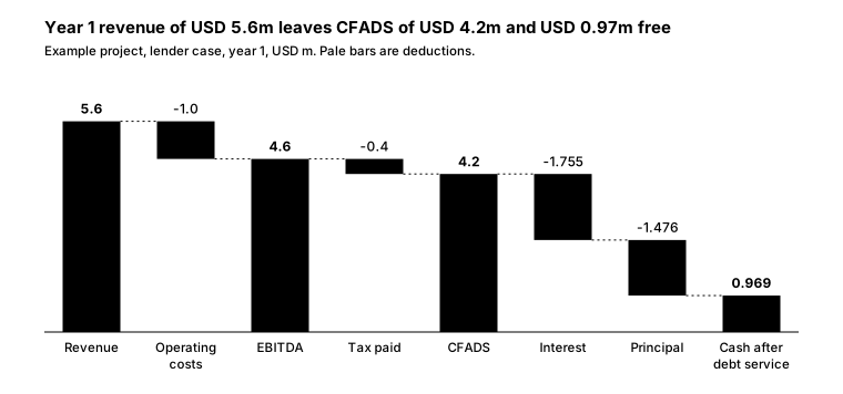
Debt service takes about three quarters of CFADS. The cash left over is the cushion that a 1.30x DSCR buys, and it funds reserves and distributions.
The common mistake is to size debt on EBITDA. At 1.30x, EBITDA of USD 4.6m would support debt service of USD 3.54m rather than USD 3.23m, about 10% too much.
What is DSCR and what counts as debt service?
DSCR (debt service cover ratio) is CFADS for a period divided by the scheduled debt service for the same period. Forvis Mazars defines it this way. A DSCR of 1.30x means the project earned USD 1.30 of CFADS for each USD 1.00 owed to lenders.
In year 1 of the example, CFADS of USD 4.2m covers interest of USD 1.755m and principal of USD 1.476m. DSCR is 1.30x.
Debt service is scheduled interest plus scheduled principal. Forvis Mazars adds that agency fees, net swap payments and other debt fees may be included, unless already counted as operating costs.
| Item | In senior debt service? | Note |
|---|---|---|
| Scheduled interest | Yes | Includes the margin |
| Scheduled principal | Yes | From the repayment schedule, not from cash actually swept |
| Net payments under the interest rate swap | Yes, unless already in operating costs | The example's 7.0% all-in rate already includes the hedge |
| Agency fee and other debt fees | Yes, unless already in operating costs | USD 40,000 a year in the example |
| Cash sweep and voluntary prepayment | No | Forvis Mazars excludes sweeps from scheduled debt service |
| Payments into the debt service reserve account | No (our reading) | A reserve transfer, not a payment to lenders |
| Subordinated debt service | Not in the senior ratio | Counted in a total DSCR, which has its own levels |
The common mistake is to count a fee on both sides. If the USD 40,000 agency fee sits in operating costs and in debt service, year 1 DSCR reads 1.28x. Counted once, on either side, it reads 1.30x.
Is DSCR periodic or annual, historic or forward-looking, average or minimum?
DSCR can be measured over one debt service period or over 12 months, and on actual results or on forecasts. Each choice gives a different number, and the term sheet says which ones are tested. Forvis Mazars notes that lenders typically assess DSCR on both a 12-month look-back and a 12-month look-forward basis.
| Variant | What it measures | What it changes in the model |
|---|---|---|
| Periodic | One debt service period, typically a quarter or a half-year | One ratio per period. Seasonal output makes it volatile. |
| Annual | CFADS and debt service summed over a 12-month window | A rolling sum on both lines before dividing |
| Historic | Actual results for the window just ended | Reads past periods. The first test may have under 12 months of history. |
| Forward-looking | Forecast CFADS for the window ahead | Reads future periods, so a weak year shows one test earlier |
| Minimum | The lowest ratio over the loan life | The figure to compare with sizing, lock-up and default levels |
| Average | The mean of the ratios over the loan life | A summary only. It hides weak years. |
With six-month periods, the annual ratio at period t sums two periods on each line:
The example uses annual periods for simplicity, so its periodic and annual ratios are the same. Real deals usually use six-month periods.
Timing matters in the downside case, where DSCR falls to 1.17x in year 3. A forward-looking test at the end of year 2 already shows 1.17x, below the 1.20x lock-up level. A historic test shows it one year later.
Average and minimum can sit far apart. In the downside case the average DSCR over 12 years is 1.26x and the minimum is 1.13x. On the level annuity alternative the average is 1.29x and the minimum is 1.26x.
What is LLCR?
LLCR (loan life cover ratio) is the net present value of CFADS to loan maturity, divided by the debt outstanding at the test date. The World Bank's PPP resource centre and the APMG PPP Guide both define it in similar words. It shows how many times the remaining cash could repay the remaining loan.
T is the final repayment period, r is the discount rate and the denominator is the opening debt balance of period t. In the example at financial close, 12 years of CFADS are worth USD 32.6m at 7.0%. Divided by debt of USD 25.07m, LLCR is 1.30x.
The discount rate. Operis states that the discount rate is the same as the interest rate, and that the two must match exactly. Operis also warns that loan documents set out interest in great detail but are typically silent on how to discount. In our reading, the rate is the all-in rate: hedged base rate plus margin.
The choice is not small. Discounting the example at the 4.0% base rate alone, without the 3.0% margin, gives 1.53x instead of 1.30x.
Opening cash and reserve balances. The plain formula adds nothing to CFADS. Some definitions add the opening cash or reserve balance to the numerator, and one published version deducts the reserve balance from the debt. Arthur Cox notes that borrowers seek to add debt service reserve account or facility amounts to the numerator.
| LLCR variant at financial close | Calculation (USD m) | Result |
|---|---|---|
| Plain | 32.59 / 25.07 | 1.30x |
| Reserve balance added to the numerator | (32.59 + 1.62) / 25.07 | 1.36x |
| Reserve balance deducted from the debt | 32.59 / (25.07 - 1.62) | 1.39x |
The table assumes the USD 1.62m debt service reserve is fully funded on day one. The common mistake is to add a balance that the definition does not mention.
What is PLCR and what is the tail?
PLCR (project life cover ratio) is the net present value of CFADS to the end of the project's life, divided by the debt outstanding. The APMG PPP Guide and SumProduct both describe it in similar words. The tail is the period between loan maturity and the end of the asset's life.
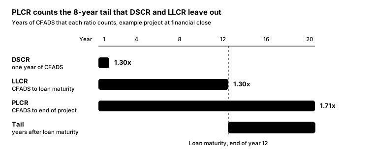
The tail is why PLCR is never lower than LLCR on the same debt. In our reading, its purpose is room to restructure: if cash flows fall for long, lenders can postpone the loan maturity.
In our reading, the end date N should be the end of contracted revenue unless the definition says otherwise. In the example that is the end of the 20-year power purchase agreement.
Why does a sculpted loan have LLCR equal to DSCR at the start?
A sculpted loan sets debt service in every period to CFADS divided by the target DSCR. The loan is the present value of that debt service at the loan rate. Substituting one into the other shows that LLCR equals the target.
In the example k is 1.30x, so LLCR is 1.30x at financial close and at every later date in the lender's case. This is arithmetic, not a market convention. It holds only if the discount rate equals the loan rate and nothing is added to the numerator.
More generally, LLCR is an average of the remaining yearly DSCRs, weighted by the present value of each year's debt service. On the level annuity alternative, LLCR at financial close is still 1.30x, while yearly DSCR runs from 1.33x down to 1.26x.
The two ratios part company when cash flows change after the loan is sized. In the downside case the debt service is fixed, but CFADS is lower in years 3 to 6.
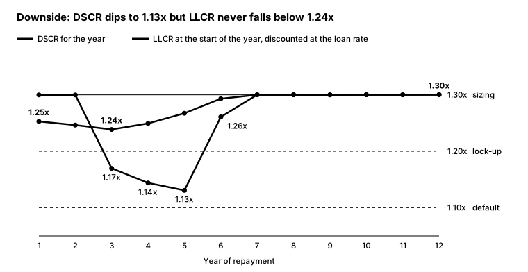
LLCR barely moves because it averages four weak years with eight normal ones. DSCR falls through the 1.20x lock-up level for three years, so a yearly DSCR test catches what an LLCR test would miss.
How do you model it?
Model each ratio as its own block of rows, built from the wording of the definition. The steps below are our method, in order.
- Copy the definitions of CFADS, debt service, DSCR and LLCR into the assumptions sheet, word for word. Mark every named item as in or out.
- Build CFADS with one signed row per item in the definition, on a cash basis. Use the same period length as the repayment dates.
- Build debt service from scheduled interest and scheduled principal. Add fees and hedge payments only if the definition names them.
- Calculate periodic DSCR as CFADS over debt service, and return a blank where debt service is nil. For an annual ratio, sum each line over the window first, then divide.
- Add separate rows for the historic and the forward-looking test. Each reads back or ahead by the window the term sheet states.
- Calculate the LLCR numerator backwards from the final repayment period, using the recursion below. Divide by the opening debt balance, and add a cash or reserve balance only if the definition says so.
- Calculate PLCR with the same recursion, started from the last period of the project's life.
- Report the minimum and the average of each ratio over the loan life. Compare the minimum with the sizing, lock-up and default levels.
- Check the result. On a sculpted loan in the lender's case, LLCR must equal the target DSCR in every period.
The recursion uses each period's own rate, so it still works when the margin steps up or the hedge is partial. With six-month periods, r is the six-month rate, calculated the same way as the interest.
What are the common mistakes?
Most errors come from using a textbook formula where the term sheet has its own. The figures below are from the example.
- Using EBITDA as CFADS. EBITDA ignores tax, capital expenditure and cash timing. In year 1 it overstates the cash by USD 0.4m.
- Including balances and non-cash items. Forvis Mazars lists depreciation, cash balances and reserve account balances as common errors in CFADS.
- Counting a fee on both sides. An agency fee in operating costs and in debt service turns 1.30x into 1.28x.
- Putting a cash sweep in debt service. A sweep is not scheduled debt service, so it would push the ratio down in the project's best years.
- Discounting LLCR at the wrong rate. The base rate without the margin gives 1.53x instead of 1.30x.
- Dividing by the closing balance. LLCR for a period uses the opening balance. Using the year 1 closing balance of USD 23.59m gives 1.38x.
- Running LLCR to the wrong date. Counting CFADS to year 20 gives the PLCR of 1.71x, not the LLCR.
- Reporting only the average. The downside case averages 1.26x, yet three years sit below the 1.20x lock-up level.
- Mixing period lengths. An annual CFADS over one six-month debt payment roughly doubles the ratio.
Frequently asked questions
Is CFADS before or after tax?
CFADS is after tax paid. Forvis Mazars calculates it by netting revenue, operating costs, capital expenditure, tax and working capital adjustments. It is tax actually paid in the period, not the accounting tax charge.
Is 1.30x a standard DSCR?
There is no single standard. Forvis Mazars describes a target of around 1.30x as common for contracted infrastructure, and adds that lenders set different levels by sector and risk. The example uses 1.30x as an invented figure, not as a market norm.
Which discount rate does LLCR use?
LLCR uses the interest rate on the debt. Operis states that the discount rate and the interest rate must match exactly. If the term sheet is silent, ask the lender to confirm the rate and the timing convention.
Why is LLCR the same as DSCR in my model?
The loan is probably sculpted to a constant DSCR. Debt service is then CFADS divided by the target, and the loan is its present value, so LLCR equals the target. The two differ once you run a sensitivity or use another repayment profile.
Is PLCR always higher than LLCR?
PLCR is higher whenever the project earns positive CFADS after loan maturity. In the example the eight-year tail lifts the ratio from 1.30x to 1.71x. With no tail the two are equal.
Do the cover ratios decide the size of the loan?
They can. In the example the 1.30x DSCR supports USD 25.1m of debt, below the USD 28.0m that the 70:30 gearing cap allows. The article "The cover ratio ladder" explains how the sizing, lock-up and default levels work together.
Sources
Pages opened on 4 October 2026 and checked again on 5 October 2026. The example project is invented and has no source.
- CFADS: Cash Flow Available for Debt Service, Forvis Mazars. How CFADS is calculated, the name CADS, the comparison with EBITDA, and the items wrongly included (depreciation, cash balances, reserve balances).
- Debt Service Coverage Ratio (DSCR): formula, meaning and use in project finance, Forvis Mazars. DSCR formula, what debt service includes, periodic and annual ratios, look-back and look-forward tests, and the remark on 1.30x.
- Cash Flow Available For Debt Service (CFADS), Corporate Finance Institute. The build of CFADS from customer receipts and the name CADS.
- Loan Life Cover Ratio: A First Principles Explanation, Operis, August 2018. LLCR formula, the rule that the discount rate matches the interest rate, and the warning that documents are typically silent on discounting.
- 8.1 Measuring Commercial Feasibility, APMG PPP Certification Guide. Definitions of LLCR and PLCR.
- Key Issues in Developing Project Financed Transactions, World Bank Public-Private Partnership Resource Center. Definition of LLCR.
- Debt Sculpting, SumProduct. PLCR formula, and LLCR as PLCR restricted to the debt period.
- Loan Life Cover Ratio (LLCR): Formula, Calculation & Requirements, Ryan O'Connell Finance. The published variant that deducts the reserve balance from the debt.
- Arc Of The (Financial) Covenant: Issues For Project And Real Estate Finance, Arthur Cox, published on Mondaq, May 2021. Borrowers seeking to add debt service reserve amounts to the LLCR numerator.